形函数

形函数是定义在参考单元上的多项式插值函数，其主要作用包括

• 实现参考单元到物理单元的映射

• 对单元内部的场变量进行插值，例如，对位移场插值 \(u(x,y)=\sum u_{i}N_{i}(x,y)\)

形函数需要满足特定的数学性质，以确保插值的正确性和数值计算的稳定性

• 插值性：\(N_{i}(\xi_{j}, \eta_{j}) = \delta_{ij}\)

• 单位分解性：\(\sum_{i=1}^{n}N_{i}(\xi, \eta) \equiv 1\)

• 连续性：在相邻单元边界处满足 \(C^{0}\) 连续

三角形单元

三节点 Lagrange 元

考虑二维空间中具有如下形式的函数：

\[ \phi = c_{1} + c_{2}\xi + c_{3}\eta, \]

因此需要 3 个形函数（基函数）

Fig. 6 三角形单元上的线性形函数

六节点 Lagrange 元

考虑二维空间中具有如下形式的函数：

\[ \phi = c_{1} + c_{2}\xi + c_{3}\eta + c_{4}\xi\eta + c_{5}\xi^2 + c_{6}\eta^2, \]

因此需要 6 个形函数（基函数）

Fig. 7 三角形单元上的二次形函数

四边形单元

四节点 Lagrange 元

考虑二维空间中具有如下形式的函数：

\[ \phi(\xi, \eta) = c_1 + c_2 \xi + c_3 \eta + c_4 \xi \eta,\]

因此需要 4 个形函数（基函数）

Fig. 8 四边形单元上的双线性形函数

九节点 Lagrange 单元

考虑二维空间中具有如下形式的函数：

\[ \phi = c_1 + c_2 \xi + c_3 \eta + c_4 \xi \eta + c_5 \xi^2 + c_6 \eta^2 + c_7 \xi^2 \eta + c_8 \xi \eta^2 + c_9\xi^2\eta^2, \]

因此需要 9 个形函数（基函数）

Fig. 9 四边形单元上的 9 节点二次形函数

八节点 Serendipity 单元

考虑二维空间中具有如下形式的函数：

\[ \phi = c_1 + c_2 \xi + c_3 \eta + c_4 \xi \eta + c_5 \xi^2 + c_6 \eta^2 + c_7 \xi^2 \eta + c_8 \xi \eta^2, \]

因此需要 8 个形函数（基函数）

Fig. 10 四边形单元上的 8 节点二次形函数

面积坐标

在有限元方法中，对于三角形或四面体等单纯形单元，通常采用面积坐标系（或称体积坐标系）来构造形函数。这种方法基于单纯形单元的几何特性，具有显著的几何优势。其核心思想是通过空间点与单纯形顶点相关联的子单纯形（如边、面或体）的归一化面积或体积比例来定义形函数的分量

Fig. 11 面积坐标系

面积坐标为

\[\begin{split} \begin{equation} \begin{aligned} L_{1}&=\frac{S_{\Delta{PP_{2}P_{3}}}}{S_{\Delta{P_{1}P_{2}P_{3}}}},\\ L_{2}&=\frac{S_{\Delta{PP_{3}P_{1}}}}{S_{\Delta{P_{1}P_{2}P_{3}}}},\\ L_{3}&=\frac{S_{\Delta{PP_{1}P_{2}}}}{S_{\Delta{P_{1}P_{2}P_{3}}}}. \end{aligned} \end{equation} \end{split}\]

在使用面积坐标（或体积坐标）构造形函数时，形函数的定义独立于三角形或四面体的具体几何形状，因此能够避免显式的参考单元到物理单元的映射

线性单元

线性单元的形函数与面积坐标直接对应

Fig. 12 面积坐标下三角形单元上的二次形函数

二次单元

线性单元的形函数与面积坐标直接对应

Fig. 13 面积坐标下三角形单元上的二次形函数

Note

在参考三角形中，面积坐标与自然坐标的形函数具有等价性。具体而言， 在参考三角形中，有 \(\xi=L_{2}\)，\(\eta=L_{3}\)，而 \(1-\xi-\eta = 1 - L_{2} - L_{3} = L_{1}\)

形函数图例

Fig. 14 一维线性形函数和二次形函数

Fig. 15 二维三角形线性形函数和二次形函数

Fig. 16 二维四边形线性形函数和二次形函数

Show code cell content Hide code cell content

import numpy as np
import matplotlib.pyplot as plt
from mpl_toolkits.mplot3d import Axes3D

# 一维单元形函数
def plot_1d_shape_functions():
    x = np.linspace(0, 1, 100)
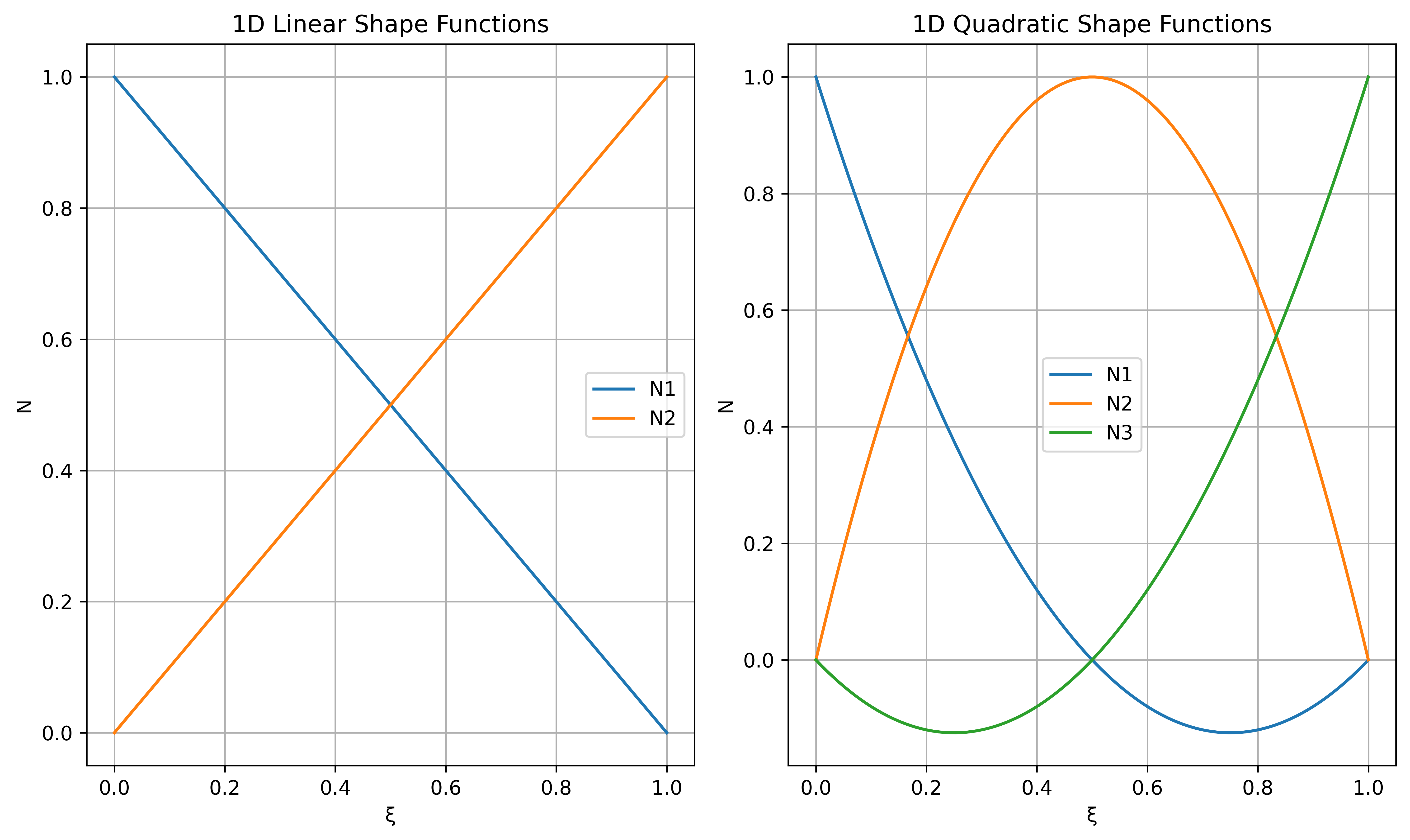
    # 一次形函数
    N1_1 = 1 - x
    N2_1 = x
    # 二次形函数
    N1_2 = (1 - x) * (1 - 2 * x)
    N2_2 = 4 * x * (1 - x)
    N3_2 = x * (2 * x - 1)

    # 节点位置
    nodes_linear = [0, 1]
    nodes_quadratic = [0, 0.5, 1]

    plt.figure(figsize=(10, 6), dpi=600)
    plt.subplot(1, 2, 1)
    plt.plot(x, N1_1, label='N1', color='#1f77b4')
    plt.plot(x, N2_1, label='N2', color='#ff7f0e')

    # 标注一次形函数的节点
    # plt.scatter([0,1],[1,0], color='#1f77b4')
    # plt.scatter([0,1],[0,1], color='#ff7f0e')

    plt.title('1D Linear Shape Functions')
    plt.xlabel('ξ')
    plt.ylabel('N')
    plt.legend()
    plt.grid()

    plt.subplot(1, 2, 2)
    plt.plot(x, N1_2, label='N1', color='#1f77b4')
    plt.plot(x, N2_2, label='N2', color='#ff7f0e')
    plt.plot(x, N3_2, label='N3', color='#2ca02c')

    # 标注二次形函数的节点
    # plt.scatter([0,0.5,1],[1,0.5,0], color='#1f77b4')
    # plt.scatter([0,0.5,1],[0,1,0], color='#ff7f0e')
    # plt.scatter([0,0.5,1],[0,0,1], color='#2ca02c')

    plt.title('1D Quadratic Shape Functions')
    plt.xlabel('ξ')
    plt.ylabel('N')
    plt.legend()
    plt.grid()
    plt.tight_layout()
    plt.show()



# 三角形单元形函数
def plot_triangle_shape_functions():
    fig = plt.figure(figsize=(12, 6), dpi=600)
    x = np.linspace(0, 1, 50)
    y = np.linspace(0, 1, 50)
    X, Y = np.meshgrid(x, y)
    mask = X + Y <= 1
    X = X[mask]
    Y = Y[mask]

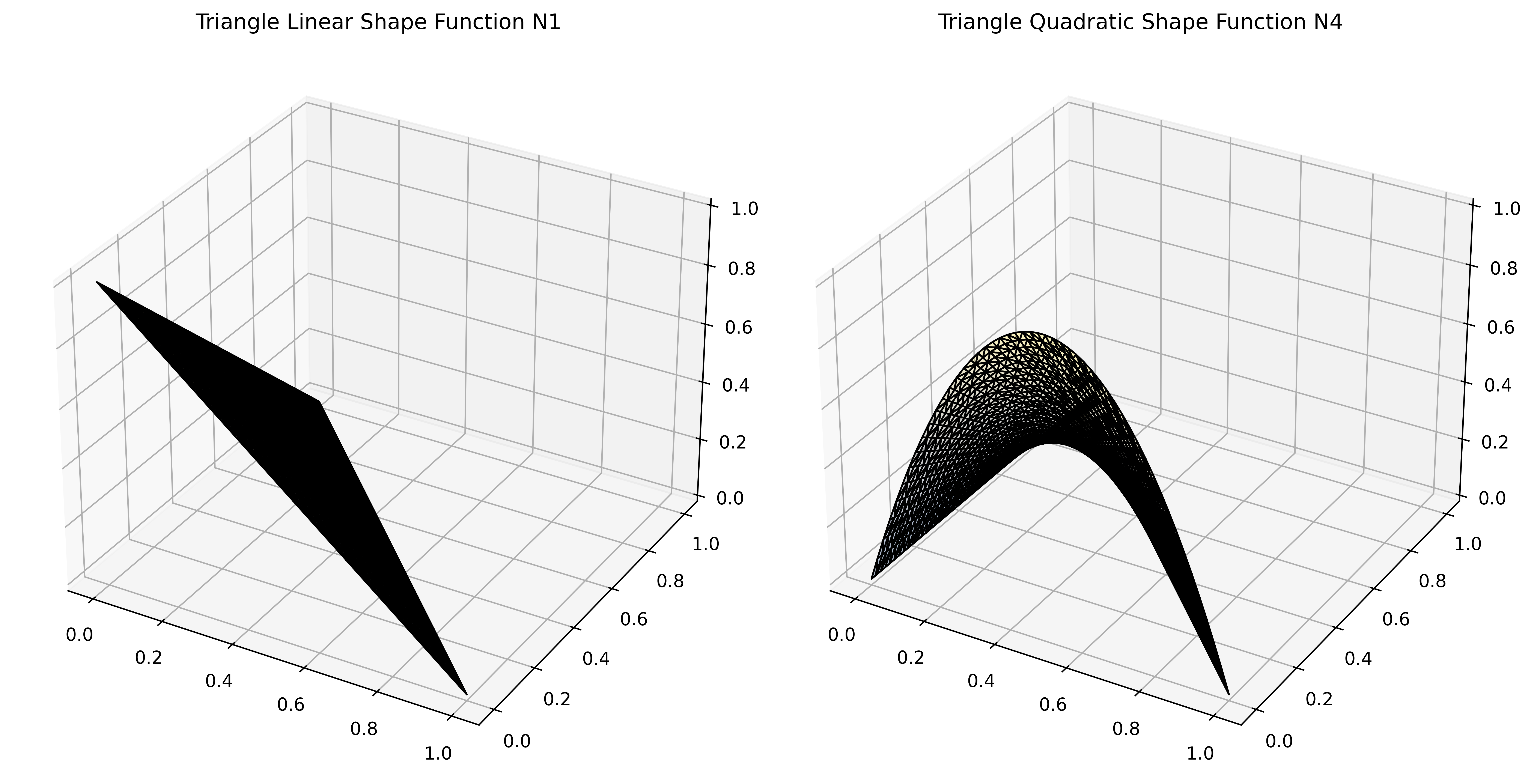
    # 一次形函数
    N1_1 = 1 - X - Y
    N2_1 = X
    N3_1 = Y

    ax1 = fig.add_subplot(121, projection='3d')
    ax1.plot_trisurf(X, Y, N1_1, cmap='cividis', edgecolor='k', alpha=0.3)
    ax1.set_title('Triangle Linear Shape Function N1')

    # 二次形函数
    N1_2 = (1 - X - Y) * (1 - 2 * (X + Y))
    N2_2 = X * (2 * X - 1)
    N3_2 = Y * (2 * Y - 1)
    N4_2 = 4 * X * (1 - X - Y)
    N5_2 = 4 * X * Y
    N6_2 = 4 * Y * (1 - X - Y)

    ax2 = fig.add_subplot(122, projection='3d')
    ax2.plot_trisurf(X, Y, N4_2, cmap='cividis', edgecolor='k', alpha=0.3)
    ax2.set_title('Triangle Quadratic Shape Function N4')

    plt.tight_layout()
    plt.show()

# 四边形单元形函数
def plot_quadrilateral_shape_functions():
    fig = plt.figure(figsize=(12, 6), dpi=600)
    xi = np.linspace(-1, 1, 50)
    eta = np.linspace(-1, 1, 50)
    XI, ETA = np.meshgrid(xi, eta)

    # 一次形函数
    N1_1 = 0.25 * (1 - XI) * (1 - ETA)
    N2_1 = 0.25 * (1 + XI) * (1 - ETA)
    N3_1 = 0.25 * (1 + XI) * (1 + ETA)
    N4_1 = 0.25 * (1 - XI) * (1 + ETA)

    ax1 = fig.add_subplot(121, projection='3d')
    ax1.plot_surface(XI, ETA, N1_1, cmap='cividis', edgecolor='k', alpha=0.3)
    ax1.set_title('Quadrilateral Linear Shape Function N1')

    # 二次形函数
    N1_2 = 0.25 * XI * ETA * (1 - XI) * (1 - ETA)
    N2_2 = 0.25 * XI * ETA * (1 + XI) * (1 - ETA)
    N3_2 = 0.25 * XI * ETA * (1 + XI) * (1 + ETA)
    N4_2 = 0.25 * XI * ETA * (1 - XI) * (1 + ETA)
    N5_2 = 0.50 * ETA * (ETA - 1) * (1 - XI**2)
    N6_2 = 0.50 * XI * (XI + 1) * (1 - ETA**2)
    N7_2 = 0.50 * ETA * (ETA + 1) * (1 - XI**2)
    N8_2 = 0.50 * XI * (XI - 1) * (1 - ETA**2)
    N9_2 = 0.50 * (1 - XI**2) * (1 - ETA**2)

    ax2 = fig.add_subplot(122, projection='3d')
    ax2.plot_surface(XI, ETA, N5_2, cmap='cividis', edgecolor='k', alpha=0.3)
    ax2.set_title('Quadrilateral Quadratic Shape Function N2')

    # 调整视角
    ax2.view_init(elev=30, azim=-60)  # 设置仰角为 45 度，方位角为 30 度

    # 去除三维面板背景（可选）
    ax1.grid(False)
    ax2.grid(False)
    for ax in [ax1, ax2]:
        ax.xaxis.pane.set_edgecolor('w')
        ax.yaxis.pane.set_edgecolor('w')
        ax.zaxis.pane.set_edgecolor('w')
        ax.xaxis.pane.set_facecolor((1.0, 1.0, 1.0, 0.0))  # 透明
        ax.yaxis.pane.set_facecolor((1.0, 1.0, 1.0, 0.0))
        ax.zaxis.pane.set_facecolor((1.0, 1.0, 1.0, 0.0))


    plt.tight_layout()
    plt.show()

# 主函数运行
if __name__ == "__main__":
    plot_1d_shape_functions()
    plot_triangle_shape_functions()
    plot_quadrilateral_shape_functions()